How to Do Error Bars in Excel?
Are you looking for a straightforward guide on how to do error bars in Excel? Then you’ve come to the right place! In this article, we will be providing you with a comprehensive step-by-step guide to adding error bars to your Excel charts and graphs. We will be discussing how to create error bars from raw data, as well as how to customize their appearance. So if you’re ready to take your Excel skills to the next level, let’s dive in!
Error bars in Excel are used to indicate the variability of the data. To add error bars in Excel:
- Open your spreadsheet in Excel.
- Select the data you want to plot, including the error bars.
- Select the ‘Chart’ tab, then click on ‘Scatter’ or ‘Line’ chart.
- Click on the ‘Design’ tab and then click on ‘Error Bars.’
- Select the type of error bar you want to use.
- Click ‘OK.’ Your chart with error bars will now be displayed.

Adding Error Bars to a Chart in Excel
Error bars are graphical representations of the variability of data and are used on graphs to indicate the error or uncertainty in a reported measurement. They give a general idea of how precise a measurement is, or conversely, how far from the reported value the true (error free) value might be. In Excel, you can add error bars to any chart type by adding a new series and then selecting the Error Bars option.
To add error bars to an existing chart, first select the chart and then click the Chart Elements button, which can be found in the upper-right corner of the chart. This will bring up a list of chart elements that you can add to your chart, including error bars. Select the Error Bars option, and then click the type of error bars you want to use. The types of error bars available are Standard Error, Percentage, Standard Deviation, and Custom.
Adding Standard Error Bars in Excel
Standard Error Bars are used to show the standard error (or standard deviation) of a data set, and can be used to compare the ranges of two or more data sets. To add standard error bars to an existing chart, select the chart and then click the Chart Elements button. Select the Error Bars option, and then select the type of error bars you want to use. Select the Standard Error option, and then click OK.
Once the error bars have been added, you can customize the appearance of the error bars. Select the chart, and then click the Chart Elements button. Select the Error Bars option, and then click the drop-down arrow next to the Error Bars option. This will open the Format Error Bars window, where you can make various adjustments to the appearance of the error bars.
Adding Percentage Error Bars in Excel
Percentage Error Bars are used to show the percentage of the difference between two or more data sets. To add percentage error bars to an existing chart, select the chart and then click the Chart Elements button. Select the Error Bars option, and then select the type of error bars you want to use. Select the Percentage option, and then click OK.
Once the error bars have been added, you can customize the appearance of the error bars. Select the chart, and then click the Chart Elements button. Select the Error Bars option, and then click the drop-down arrow next to the Error Bars option. This will open the Format Error Bars window, where you can make various adjustments to the appearance of the error bars.
Adding Standard Deviation Error Bars in Excel
Standard Deviation Error Bars are used to show the standard deviation of a data set, and can be used to compare the ranges of two or more data sets. To add standard deviation error bars to an existing chart, select the chart and then click the Chart Elements button. Select the Error Bars option, and then select the type of error bars you want to use. Select the Standard Deviation option, and then click OK.
Once the error bars have been added, you can customize the appearance of the error bars. Select the chart, and then click the Chart Elements button. Select the Error Bars option, and then click the drop-down arrow next to the Error Bars option. This will open the Format Error Bars window, where you can make various adjustments to the appearance of the error bars.
Adding Custom Error Bars in Excel
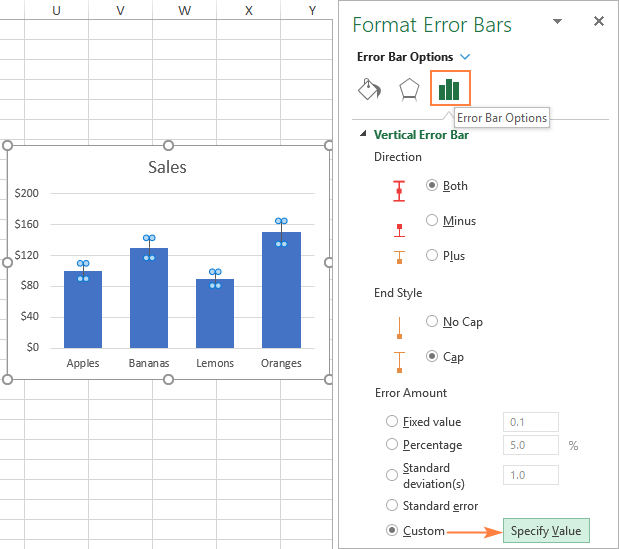
Custom Error Bars are used to show a specific value or range of values on a chart. To add custom error bars to an existing chart, select the chart and then click the Chart Elements button. Select the Error Bars option, and then select the type of error bars you want to use. Select the Custom option, and then click OK.
Once the error bars have been added, you can customize the appearance of the error bars. Select the chart, and then click the Chart Elements button. Select the Error Bars option, and then click the drop-down arrow next to the Error Bars option. This will open the Format Error Bars window, where you can make various adjustments to the appearance of the error bars.
Formatting Error Bars in Excel
Once the error bars have been added to a chart, you can customize the appearance of the error bars. Select the chart, and then click the Chart Elements button. Select the Error Bars option, and then click the drop-down arrow next to the Error Bars option. This will open the Format Error Bars window, where you can make various adjustments to the appearance of the error bars.
In the Format Error Bars window, you can adjust the color, size and line style of the error bars. You can also adjust the width of the bars, the amount of spacing between them, and the direction of the error bars. You can also add labels and a custom error message to the error bars.
Once you have adjusted the appearance of the error bars, click the OK button to apply your changes. Your error bars will now be visible on the chart.
Related Faq
What are Error Bars in Excel?
Error Bars in Excel are graphical representations of the variability of data. They are used to indicate the range of values within a set of data. Error Bars can be added to a chart or graph to show the uncertainty in a reported measurement. They can also be used to compare two or more sets of data and to show the correlation between them.
What are the Different Types of Error Bars?
Error Bars in Excel come in three different types: standard error, standard deviation, and percent error. Standard error bars display the standard error of the mean for the data set, while standard deviation bars display the standard deviation of the data set. Percent error bars display the percent error of the data set.
How to Create Error Bars in Excel?
Creating Error Bars in Excel is simple. First, select the chart or graph that you would like to add Error Bars to. Then, click on the “Chart Elements” button located in the upper right corner of the chart. From there, select “Error Bars” from the list of chart elements. After selecting “Error Bars”, select the type of error bars you would like to add from the drop-down menu. Finally, click “OK”.
How to Customize Error Bars in Excel?
Customizing Error Bars in Excel is easy. First, select the chart or graph you would like to customize. Then, click on the “Chart Elements” button located in the upper right corner of the chart. From there, select “Error Bars” from the list of chart elements. After selecting “Error Bars”, select the type of error bars you would like to customize from the drop-down menu. Finally, click “Format Error Bars”. This will open the “Format Error Bars” menu, where you can customize the color, size, and other attributes of the error bars.
How to Add Labels to Error Bars in Excel?
Adding labels to Error Bars in Excel is simple. First, select the chart or graph you would like to add labels to. Then, click on the “Chart Elements” button located in the upper right corner of the chart. From there, select “Error Bars” from the list of chart elements. After selecting “Error Bars”, select the type of error bars you would like to customize from the drop-down menu. Finally, click “Format Error Bars”. This will open the “Format Error Bars” menu, where you can add labels to the error bars by selecting the “Labels” option.
How to Change the Direction of Error Bars in Excel?
Changing the direction of Error Bars in Excel is easy. First, select the chart or graph you would like to change the direction of. Then, click on the “Chart Elements” button located in the upper right corner of the chart. From there, select “Error Bars” from the list of chart elements. After selecting “Error Bars”, select the type of error bars you would like to customize from the drop-down menu. Finally, click “Format Error Bars”. This will open the “Format Error Bars” menu, where you can change the direction of the error bars by selecting either “Up/Down Bars” or “High/Low Bars”.
How To Add Error Bars In Excel (Custom Error Bars)
Error bars can be an effective way to display data in Excel. Knowing how to do error bars in Excel can help you create clearer visuals that can be easily interpreted. Whether you’re using them to compare groups or to show possible error margins, error bars can be a useful tool. With a few simple steps, you can rapidly add error bars to any Excel chart.
Related Posts

Small businesses struggle with ERC tax credit submissions

10 Misunderstandings of the Employee Retention Credit
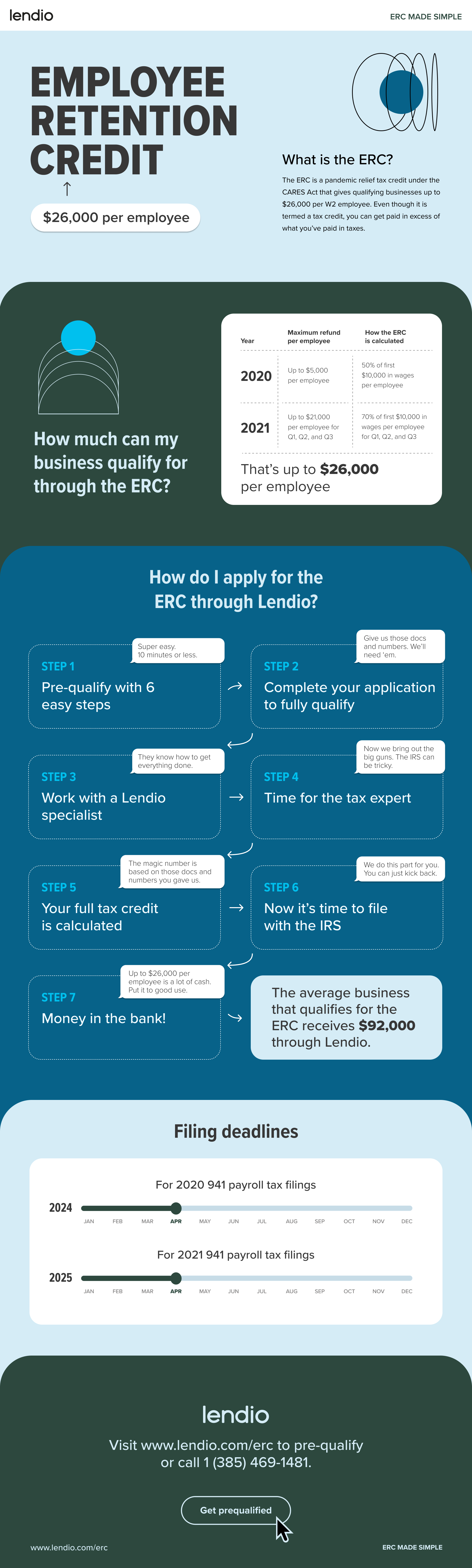
ERC Tax Credit 2023: Is the ERC tax credit still available?