How to Change Date Format on Excel?

If you’ve ever had to work with dates in Microsoft Excel, you know how confusing it can be to get your desired date format. You may be wondering how to get Excel to display the dates the way you need them. Fortunately, Excel makes it easy to change the date format to one that works for your needs. In this article, we’ll show you how to change the date format on Excel, so you can make sure your data is presented in the way you want it.

How to Customize Date Formats in Excel

Customizing the date format in Excel can be useful for when you are trying to organize data or make it easier to read. With a few simple steps you can quickly and easily change the date format in Excel. This tutorial will walk you through the basics of changing the date format in Excel.

Understanding Excel’s Date Formatting Options

Excel has a variety of date formatting options that you can choose from. These options range from displaying the date in the format of day, month, year to displaying the date in the format of month, day, year. You can also choose to display the date in a more detailed way, such as including the day of the week or the time of day.

Changing the Date Format in Excel

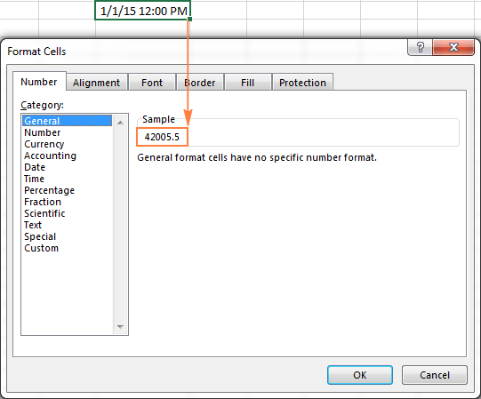
To change the date format in Excel, you will need to click on the cell or range of cells that contains the dates you want to format. Then, select the “Format Cells” option from the Home tab. In the Format Cells window, you can then select the “Date” category and then select your desired date format. Once you have selected the format, click OK to apply it to the selected cells.

Using Custom Date Formats in Excel

If you want to create a custom date format in Excel, you can also do this by selecting the “Custom” option from the list of date formatting options. This will open the “Format Cells” window where you can enter the custom formatting codes to create the date format you want.

Using Formulas to Automatically Format Dates in Excel

You can also use formulas in Excel to automatically format dates. For example, you can use the TEXT function to convert a date in one format to a date in another format. You can also use the DATEVALUE function to convert a text string to a date.

Using Conditional Formatting to Automatically Format Dates in Excel

You can also use conditional formatting in Excel to automatically format dates. This can be done by selecting the cells that you want to apply the formatting to and then selecting the “Conditional Formatting” option from the Home tab. Then, select the “Highlight Cells Rules” option and then select the “Date Occurring” option. This will open the “Conditional Formatting Rules” window where you can select the date format you want to apply.

Using VBA to Automatically Format Dates in Excel

You can also use Visual Basic for Applications (VBA) to automatically format dates in Excel. This can be done by creating a macro that will loop through the selected range of cells and apply the desired date format. You can then run the macro when you need to automatically format dates in Excel.

Using the Format Painter to Apply Date Formats in Excel

The Format Painter tool in Excel can be used to quickly and easily apply a certain date format to a range of cells. To use the Format Painter, select the cell with the desired date format, click the Format Painter button, and then select the cells you want to apply the format to.

Related FAQ

Q1: What is the Date Format in Excel?

Answer: Excel typically uses the default date format of “mm/dd/yyyy”, which stands for month, day, and four digit year. This is the most common format used in the United States. However, there are other formats available depending on the country or region. For example, in France the date format is “dd/mm/yyyy”, which stands for day, month, and four digit year.

Q2: How Do I Change the Date Format in Excel?

Answer: To change the date format in Excel, first select the cells that you want to change. Then, go to the Home tab and select the Number group. From there, click the small arrow on the bottom right corner of the group and select “More Number Formats”. In the new window, select the format you want from the Category list and click OK.

Q3: How Do I Create a Custom Date Format in Excel?

Answer: To create a custom date format in Excel, start by selecting the cells you want to format. Go to the Home tab and select the Number group. From there, click the small arrow on the bottom right corner of the group and select “More Number Formats”. In the new window, select the “Custom” option from the Category list. This will open the Type window, where you can create a custom date format using symbols.

Q4: How Do I Show the Day of the Week in Excel?

Answer: To show the day of the week in Excel, start by selecting the cells you want to format. Go to the Home tab and select the Number group. From there, click the small arrow on the bottom right corner of the group and select “More Number Formats”. In the new window, select the “Short Date” option from the Category list, and then select the “dddd” option from the Type list.

Q5: How Do I Show the Month as a Word in Excel?

Answer: To show the month as a word in Excel, start by selecting the cells you want to format. Go to the Home tab and select the Number group. From there, click the small arrow on the bottom right corner of the group and select “More Number Formats”. In the new window, select the “Long Date” option from the Category list, and then select the “mmmm” option from the Type list.

Q6: How Do I Show the Year in Excel?

Answer: To show the year in Excel, start by selecting the cells you want to format. Go to the Home tab and select the Number group. From there, click the small arrow on the bottom right corner of the group and select “More Number Formats”. In the new window, select the “Long Date” option from the Category list, and then select the “yyyy” option from the Type list. This will display the year in four digits.

Unable to Change Date Format in Excel ? You need to watch this | Microsoft Excel Tutorial

The ability to change the date format of your data in Excel can be a powerful tool for any user. By following the simple steps outlined in this article, you can quickly and easily customize your data to your desired format. Whether you’re looking to change the display of a single cell or an entire range of cells, the versatility of Excel can help you make the changes you need in no time.