How to Divide in Excell?
Excel is an incredibly powerful tool that can help you save time and make complex calculations and data analysis easier. If you’re looking to learn how to divide in Excel, you’ve come to the right place. In this guide, you’ll learn how to divide in Excel quickly and easily. We’ll walk through the different methods of division, as well as tips and tricks to make your division calculations as efficient as possible. So, let’s dive in and learn how to divide in Excel.
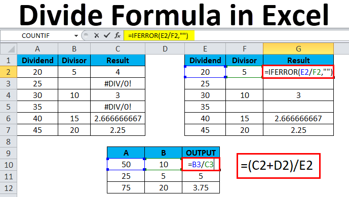
To divide in Excel, use the division symbol, which is the forward slash character ( / ).
- Start by entering the formula you want to use to divide in the cell where you want the answer to appear.
- For example, if you want to divide 10 by 2, enter the formula =10/2
- Press the Enter key on your keyboard to complete the formula.
- The result of the division, 5, will appear in the cell.
Divide in Excel with Simple Steps
Division is a fundamental math operation that allows you to find the number of times one number is contained in another. This can be done in Excel by using the division operator (/) to calculate the result of a division equation. Excel also offers a variety of functions and tools that can be used to divide numbers and cells, such as the QUOTIENT(), MOD(), and DIVIDE() functions. In this article, we will take a look at how to divide in Excel with simple steps.
Division in Excel can be done with the use of a simple equation or formula. To divide two numbers in Excel, simply enter the equation in a cell and Excel will calculate the result. For example, if you enter the equation “=10/2” in cell A1, Excel will display the result “5” in that cell.
In addition to using a simple equation to divide in Excel, you can also use the QUOTIENT(), MOD(), and DIVIDE() functions. The QUOTIENT() function is used to find the integer portion of a division equation, while the MOD() function returns the remainder of a division equation. The DIVIDE() function is used to divide two numbers and return the result as a percentage.
Use the QUOTIENT() Function to Divide in Excel
The QUOTIENT() function can be used to divide two numbers and return the integer portion of the result. To use the QUOTIENT() function, you need to enter the equation in a cell, followed by two arguments separated by a comma. The first argument is the number that is being divided, while the second argument is the number that is being divided by. For example, if you enter the equation “=QUOTIENT(10,2)” in cell A1, Excel will display the result “5” in that cell.
The QUOTIENT() function can also be used to divide an array of numbers. To do this, you need to enter the equation in a cell, followed by two arguments separated by a comma. The first argument is the array of numbers that is being divided, while the second argument is the number that is being divided by. For example, if you enter the equation “=QUOTIENT(A2:A5,2)” in cell A1, Excel will display the result “5,4,3,2” in that cell.
Use QUOTIENT() in Conditional Formatting
The QUOTIENT() function can also be used in Excel’s Conditional Formatting feature. To use the QUOTIENT() function in Conditional Formatting, you need to select the cells that you want to apply the formatting to, and then click the “Conditional Formatting” button in the “Home” tab. Next, select “New Rule” from the drop-down menu and choose “Format only cells that contain” from the “Select a Rule Type” list.
In the “Edit the Rule Description” box, select “Format only cells with” from the drop-down menu and then select “QUOTIENT” from the formula list. Finally, enter the formula in the “Value or Formula” section. For example, if you enter the formula “=QUOTIENT(A2:A5,2)”, Excel will apply the formatting to cells that contain the result “5,4,3,2”.
Use the MOD() Function to Divide in Excel
The MOD() function can be used to divide two numbers and return the remainder of the result. To use the MOD() function, you need to enter the equation in a cell, followed by two arguments separated by a comma. The first argument is the number that is being divided, while the second argument is the number that is being divided by. For example, if you enter the equation “=MOD(10,2)” in cell A1, Excel will display the result “0” in that cell.
The MOD() function can also be used to divide an array of numbers. To do this, you need to enter the equation in a cell, followed by two arguments separated by a comma. The first argument is the array of numbers that is being divided, while the second argument is the number that is being divided by. For example, if you enter the equation “=MOD(A2:A5,2)” in cell A1, Excel will display the result “1,0,1,0” in that cell.
Use MOD() in Conditional Formatting
The MOD() function can also be used in Excel’s Conditional Formatting feature. To use the MOD() function in Conditional Formatting, you need to select the cells that you want to apply the formatting to, and then click the “Conditional Formatting” button in the “Home” tab. Next, select “New Rule” from the drop-down menu and choose “Format only cells that contain” from the “Select a Rule Type” list.
In the “Edit the Rule Description” box, select “Format only cells with” from the drop-down menu and then select “MOD” from the formula list. Finally, enter the formula in the “Value or Formula” section. For example, if you enter the formula “=MOD(A2:A5,2)”, Excel will apply the formatting to cells that contain the result “1,0,1,0”.
Use the DIVIDE() Function to Divide in Excel
The DIVIDE() function can be used to divide two numbers and return the result as a percentage. To use the DIVIDE() function, you need to enter the equation in a cell, followed by two arguments separated by a comma. The first argument is the number that is being divided, while the second argument is the number that is being divided by. For example, if you enter the equation “=DIVIDE(10,2)” in cell A1, Excel will display the result “50%” in that cell.
The DIVIDE() function can also be used to divide an array of numbers. To do this, you need to enter the equation in a cell, followed by two arguments separated by a comma. The first argument is the array of numbers that is being divided, while the second argument is the number that is being divided by. For example, if you enter the equation “=DIVIDE(A2:A5,2)” in cell A1, Excel will display the result “50%,25%,16.67%,12.5%” in that cell.
Use DIVIDE() in Conditional Formatting
The DIVIDE() function can also be used in Excel’s Conditional Formatting feature. To use the DIVIDE() function in Conditional Formatting, you need to select the cells that you want to apply the formatting to, and then click the “Conditional Formatting” button in the “Home” tab. Next, select “New Rule” from the drop-down menu and choose “Format only cells that contain” from the “Select a Rule Type” list.
In the “Edit the Rule Description” box, select “Format only cells with” from the drop-down menu and then select “DIVIDE” from the formula list. Finally, enter the formula in the “Value or Formula” section. For example, if you enter the formula “=DIVIDE(A2:A5,2)”, Excel will apply the formatting to cells that contain the result “50%,25%,16.67%,12.5%”.
Few Frequently Asked Questions
Q1. How can I divide two cells in Excel?
A1. You can divide two cells in Excel by using the ‘/’ operator. To do this, start by selecting the two cells you want to divide. Then, enter the ‘/’ operator into the formula bar and click enter. Excel will then divide the two cells and show the result in the cell you selected. You can also use the ‘/’ operator with multiple cells, for example: A2/B2/C2. This will divide the values in cells A2, B2 and C2 and show the result in the cell you selected.
Q2. Can I use parentheses in Excel formulas?
A2. Yes, you can use parentheses in Excel formulas. Parentheses are used to indicate which operations are performed first in a formula. For example, if you have the formula A1+B1/C1, Excel will divide B1 and C1 before adding A1. However, if you use parentheses and enter the formula (A1+B1)/C1, Excel will first add A1 and B1, then divide the result by C1. This is useful for ensuring that Excel calculates the formula in the order you want it to.
Q3. How do I divide a range of cells in Excel?
A3. You can divide a range of cells in Excel by using the ‘/’ operator and the SUM function. To do this, start by selecting the range of cells you want to divide. Then, enter the ‘/’ operator into the formula bar followed by the SUM function. For example: =SUM(A1:A5)/5. This will take the sum of all the values in the range A1 to A5 and divide it by 5. The result will be shown in the cell you selected.
Q4. How do I divide a column of cells in Excel?
A4. You can divide a column of cells in Excel by using the ‘/’ operator and the SUM function. To do this, start by selecting the column of cells you want to divide. Then, enter the ‘/’ operator into the formula bar followed by the SUM function. For example: =SUM(A1:A5)/5. This will take the sum of all the values in the column A1 to A5 and divide it by 5. The result will be shown in the cell you selected.
Q5. Is there a shortcut for dividing cells in Excel?
A5. Yes, there is a shortcut for dividing cells in Excel. You can use the ‘Ctrl + /’ shortcut to divide two cells in Excel. To do this, select the two cells you want to divide, then press the ‘Ctrl + /’ keys on your keyboard. Excel will then divide the two cells and show the result in the cell you selected.
Q6. How do I divide a formula in Excel?
A6. You can divide a formula in Excel by using the ‘/’ operator. To do this, start by entering the formula into the formula bar. Then, divide the formula by adding the ‘/’ operator where appropriate. For example, if you want to divide the formula A1+B1/C1, you would enter (A1+B1)/C1 into the formula bar. Excel will then divide the formula and show the result in the cell you selected.
Excel is a powerful tool for performing calculations and analysing data. Dividing data in Excel is a simple task that can be done in a few steps. By following the steps outlined in this article, you can easily divide your data in Excel and use the results for further analysis. So, if you ever find yourself in need of dividing data, you can now do it with confidence in Excel.
Related Posts

Small businesses struggle with ERC tax credit submissions

10 Misunderstandings of the Employee Retention Credit
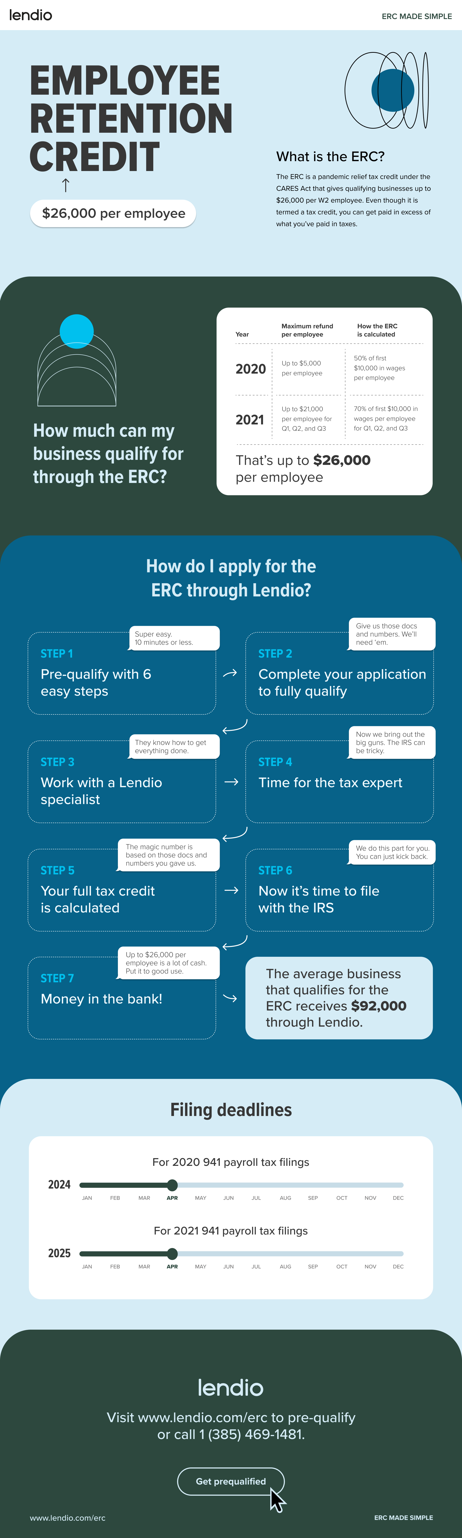
ERC Tax Credit 2023: Is the ERC tax credit still available?