How to Use Hlookup Function in Excel?
Are you looking for a quick and easy way to find data in Excel? Look no further than the Hlookup function. This powerful tool can help you quickly locate the data you need from a large dataset. In this article, you’ll learn how to use the Hlookup function, as well as its advantages and disadvantages. With a few simple steps, you’ll be able to quickly and accurately find the data you need in Excel.
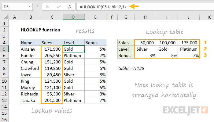
Hlookup is a function in Microsoft Excel that allows you to search for a value in the top row of a table and return a value in the same column from any row you specify. To use the Hlookup function in Excel:
- Start by opening your Excel spreadsheet and selecting the cell where you want to place the Hlookup result.
- Type the “=Hlookup” formula into the selected cell.
- In the parentheses that follow the formula, enter the following information: the value you are searching for, the table array, the row number, and the column number.
- Press Enter to complete the formula and display the result.

What is Hlookup Function & How to Use it in Excel?
The Hlookup function (or horizontal lookup) is a powerful tool in Microsoft Excel that allows you to quickly and easily search for data in a row or column. It can be used to look up values from a table, compare values from a range of cells, or return a value from a column. This article will explain how to use the Hlookup function in Excel, as well as provide some useful tips and tricks for getting the most out of the Hlookup function.
The Hlookup function is a powerful tool that can be used to look up values in a table or range of cells. It works by searching horizontally across a row or column of data to find a specific value. The function returns the value associated with the value you specify in the search argument. For example, if you want to look up the value associated with a certain name, you can use the Hlookup function to return the value associated with that name in the table.
Syntax of Hlookup Function
The syntax of the Hlookup function is as follows: Hlookup(lookup_value, lookup_range, column_number, match_type). The lookup_value argument specifies the value you are looking for. The lookup_range argument specifies the range of cells where the lookup_value can be found. The column_number argument specifies the column number of the cell containing the value you are looking for. Finally, the match_type argument specifies whether you want an exact or approximate match when searching for the lookup_value.
How to Use the Hlookup Function in Excel
Using the Hlookup function in Excel is relatively straightforward. First, you will need to select the range of cells in which you want to search for the specified value. Next, enter the Hlookup function in the formula bar and specify the lookup_value, lookup_range, column_number, and match_type. Finally, press enter to execute the Hlookup function.
Examples of How to Use Hlookup Function in Excel
To illustrate how to use the Hlookup function in Excel, let’s take a look at two examples. The first example will look up the value associated with a name in a table. The second example will compare two values from a range of cells and return the value associated with the second value.
Example 1: Look Up a Value in a Table
In this example, we will look up the value associated with the name “John Smith” in a table. We can do this using the following formula: Hlookup(“John Smith”, A1:D7, 2, FALSE). This formula will search the range of cells A1 to D7 for the value “John Smith” and return the value associated with it from the second column.
Example 2: Compare Two Values from a Range of Cells
In this example, we will compare two values from a range of cells and return the value associated with the second value. We can do this using the following formula: Hlookup(A1, B1:D7, 3, TRUE). This formula will search the range of cells B1 to D7 for the value in cell A1 and return the value associated with it from the third column.
Tips & Tricks for Using the Hlookup Function in Excel
Here are a few tips and tricks for using the Hlookup function in Excel:
Tip 1: Specify the Range Accurately
When specifying the lookup_range argument, make sure to specify the range accurately. If the lookup_range is not accurate, the Hlookup function may not return the desired result.
Tip 2: Use Wildcards When Searching for Values
You can use wildcards (i.e. the asterisk (*) or question mark (?)) when searching for values in the lookup_value argument. This can be useful for searching for values that may have a few different variations.
Tip 3: Use the Match_type Argument for an Exact Match
If you want the Hlookup function to return an exact match, you can use the match_type argument. Set the match_type argument to TRUE for an exact match or FALSE for an approximate match.
Few Frequently Asked Questions
The HLOOKUP function in Excel is an invaluable tool for quickly and efficiently finding data in large datasets. It can be a bit tricky to learn, but with a little practice and patience, you’ll be a pro in no time. Whether you’re a data analyst, a spreadsheet enthusiast, or just looking for an easier way to find data in Excel, the HLOOKUP function is a great choice. With its powerful search capabilities, you can quickly and easily access the data you need to make informed decisions.
Related Posts

Small businesses struggle with ERC tax credit submissions

10 Misunderstandings of the Employee Retention Credit

ERC Tax Credit 2023: Is the ERC tax credit still available?